5 min Recap for Andrew Ng Deep Learning Specialization-Course 2

Week-1

Building a ML model is an iterative process in which multiple models needs to be tried and tested and then deployed.

The first first step is to divide the data-set into 3 parts

• Train Set
• Hold-out/Cross Validation Set/Dev Set-It is used to iterate between the models and tuning of hyperparameters.
• Test Set-It is used to give the unbiased performance of the model.

If the data is large then data needs to divided in the ratio of 98%,1% and 1% respectively.

Dev and Test set needs to come from same distribution

If the model is underfitting the data ,if it contains high error rate then it is said to be Have high bias.If it is overfitting the data ,then it is said to be high variance case.

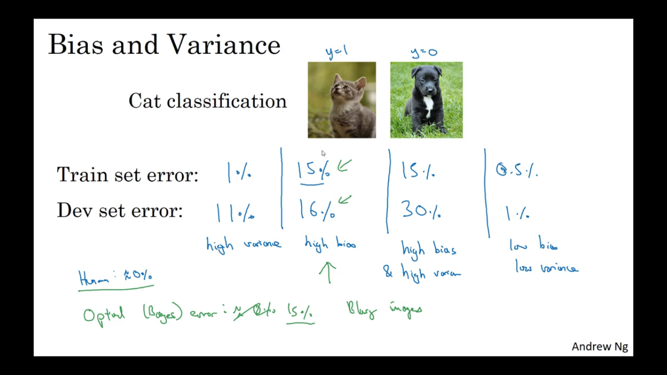
The thumb rule for building a ML model is check if it has-

• High Bias-then build bigger network or train longer
• High Variance(dev set performance)-Use More data,Use Regularization

Regularization

Helps to reduce overfitting and hence high variance.

Regularization is done by adding following values-

The main intuition behind this is when we add a term to the loss function ,we basically are penalizing the neural network for having high values of W ,so if the value of W is incentivize ,if value is more comparable to 0,which will practically zero out the output of many hidden units.

There is another technique of Regularization called Drop-Out in which in each layer there is a certain probability of removing a node and hence reducing neural network to a shorter one.

Drop-out is implemented as below-

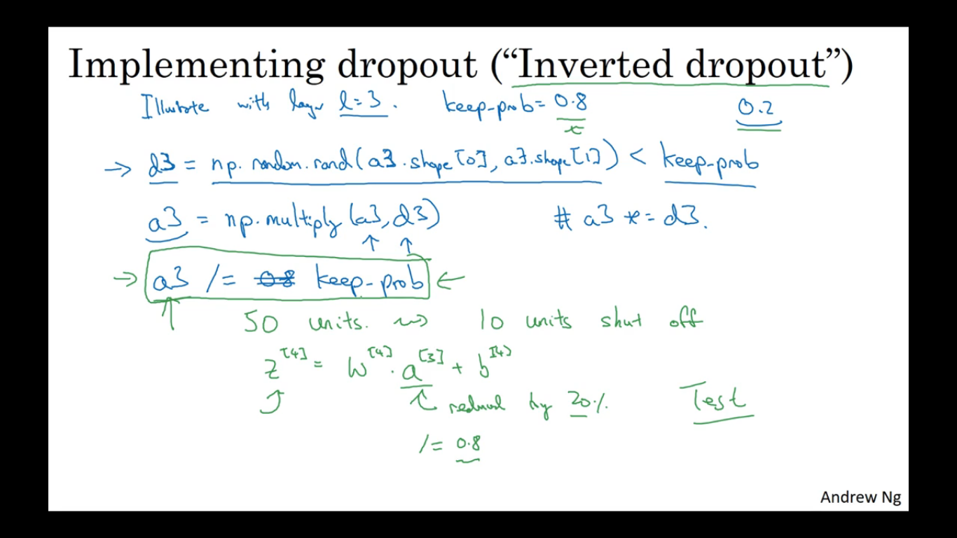
Drop out works because it makes all the nodes has to spread out their weights as any node can be removed so it will reduce overfitting.

There are other regularization methods-

• Data augmentation-By flipping the images or cropping the images.

While training a neural network,an efficient way to speed up the process is to normalize the input variables.

Gradient step will require many steps to oscillate back and forth in case of non-normalized input as distribution will not be symmetric.

While training ,values of parameters can become very large(exploding gradient) or very small(vanishing gradients).

To avoid the problem of vanishing/exploding gradient ,weight initialization is used.Following initialization are being used-

Week-2

Instead of passing all the training example in a single pass,there is a technique in which training set is divided into smaller sizes called
mini- batches and then processed .
One pass throug a mini-batch is called epoch

In Batch gradient-descent ,the cost function is bound to decrease with every iteration as it is done on all the examples but in the case of mini-batch gradient-descent ,it is not necessary as it operates on different training examples.

Mini-batch size should be between 1 (called stochastic gradient-descent) and m(total number of training examples) because

• If size is 1 then speed will be almost slow as one will processing each training examples
• Size = m is same as batch gradient descent ,hence too much slow.
  If data-set size is small then batch-gradient descent should be used otherwise batches of the power of 2 must be used.

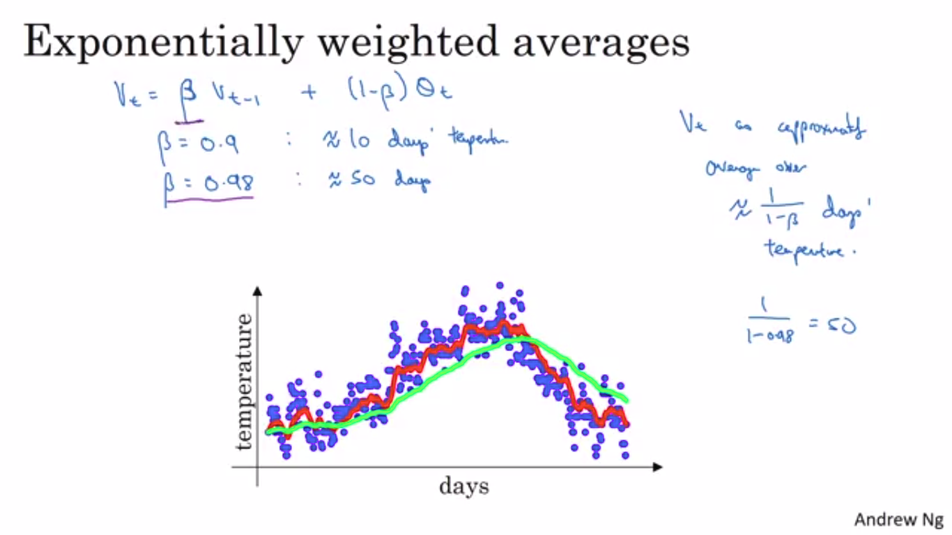
Exponentially Weighted Moving Average
The main prerequisite to understand optimization algorithms better than the gradient descent is Exponentially Weighted Average which is used to calculate local average.

In order to calculate EWPA,
v_current=beta*v_prev+(1-beta)*current_y-axis_value

beta value monitor the smoothness of the curve,more the value closer to 1 ,smoother the curve is as it is averaging over the larger window
EWMA smoothens the
In order to remove the initial bias ,bias correction is introduced.

Gradient Descent with Momentum
In Gradient Descent with momentum ,in order to damp the oscillations ,EWMA is introduced.
While computing dW and db
V_dW=beta*V_dW+(1-beta)*dW
And hence
W=W-alpha*V_dW
similarly dB is calculated.

RMS Prop
RMS prop is used to dampen the vertical oscillations and fasten the horizontal oscillation.The main intuition behind RMS prop is ,as dw values move slowly so we’ll divide the smaller value from the W .
Similarly dB value moves faster so we’ll divide it to make B value smaller.
Equation are in the figure.Epsilon is added to prevent the equation from dividing by zero.

Adam Optimization Algorithm
Adam Optimization Algorithm is combination of Momentum and RMS Prop.First the Momentum is applied ,followed by RMS prop,bias correction is also done.
Equation given in the pic.
pic 5
Choice of hyperparameter-
Alpha-Needs to be tuned
beta_1–0.9
beta_2–0.999
Epsilon-10^-8

Learning Rate Decay
To speed up the optimization,learning rate decay is used in which initially the learning rate is faster in comparison to the end of the iteration.
As learning rate is slower so steps will be slower and it will move around the minima

There are some other Learning rate decay methods-

Local Optima
Earlier,the main problem while minimising the cost is getting struck in local optima rather than ending in global optima but now it has been researched that chances of getting struck in local optima is very-very low.
Instead ,now the main problem is of plateaus.They make learning slow.

WEEK-3

HYPERPARAMETER TUNING
Tuning of hyperparameter is a essential part in training a neural network.
Following are the default values according to Andrew Ng and they can differ for one practitioner to another.

There are basically 2 approaches in tuning hyperparameters-

• Using random value ,rather than using a grid.As using a grid will limit the number of values used,While trying random numbers can lead to testing large number of values

-Limiting the sample size by narrowing down the sample-space and then densely testing in that smaller sample-space.

Using an Appropriate Scale to pick hyperparameters
Instead of using a linear scale to pick-hyperparameters,using a logarithmic scale is much efficient and more useful.
pic-4

Pandas vs Caviar
Hyperparameters may get outdated with time for a particular problem with onset of new data or due to several other factors.So in order to avoid it ,we need to test hyperparameters regularly.
There are 2 approaches for it-

• Pandas-When resources are scarce ,train a model and test it continously after time.
• Caviar-When resources are plenty,train multiple models and choose the best fit.

BATCH NORMALISATION
Batch Normalisation is used to find the range for tuning hyperparameters and hence used to train deeper neural-network and speed up learning.
Normalisation in logistic regression consists of mainly 2 parts-

• Calculating mean and subtracting X(input vector) from it.
• Calculating variance and dividing X (input vector) from it.
  It will lead to 0-mean and Variance-1 input values.
  But in hidden layers of neural network ,we don’t always need (0,1) mean-variance so we use the constants-beta and gamma to scale the values,As we want to capitalize the property of relu function.

Here epsilon is used to prevent denominator from zeroing out.

Fitting Batch Norm into Neural Network
Batch Normalisation consists of following parts-

We can remove the variable b-vector as the Batch norm will in turn cancel out the b-term.

Why Batch-Norm Works
Batch Norm ,in case of data-distribution change helps in normalising the data,called(covariate-shift).

Neural-Network suffers from co-variate shift as the value of hidden layers changes to achieve a optimum value.

Batch Norm resolves this value by reducing the amount ,these hidden layer shifts around,as the mean and variance remains the same.It makes each layer more independent than earlier.
Also it acts as a regulariser.

While testing the neural network,as in order to calculate mean and variance(as mean and variance are calculate over the size of mini-batches),EWMA value is used of all the mini-batches.

Multiclass Classification
In order to classify multiply classes of objects,Softmax Regression is used.
In Softmax regression ,the activation function in the output layer is different.

This was 2