by on
Today’s blog post on multi-label classification with Keras was inspired from an email I received last week from PyImageSearch reader, Switaj.
Switaj writes:
Hi Adrian, thanks for the PyImageSearch blog and sharing your knowledge each week.
I’m building an image fashion search engine and need help.
Using my app a user will upload a photo of clothing they like (ex. shirt, dress, pants, shoes) and my system will return similar items and include links for them to purchase the clothes online.
The problem is that I need to train a classifier to categorize the items into various classes:
- Clothing type: Shirts, dresses, pants, shoes, etc.
- Color: Red, blue, green, black, etc.
- Texture/appearance: Cotton, wool, silk, tweed, etc.
I’ve trained three separate CNNs for each of the three categories and they work really well.
Is there a way to combine the three CNNs into a single network? Or at least train a single network to complete all three classification tasks?
I don’t want to have to apply them individually in a cascade of if/else code that uses a different network depending on the output of a previous classification.
Thanks for your help.
Switaj poses an excellent question:
Is it possible for a Keras deep neural network to return multiple predictions?
And if so, how is it done?
To learn how to perform multi-label classification with Keras, just keep reading.
Multi-label classification with Keras
Today’s blog post on multi-label classification is broken into four parts.
In the first part, I’ll discuss our multi-label classification dataset (and how you can build your own quickly).
From there we’ll briefly discuss
We’ll then take our implementation of
Finally, we’ll wrap up today’s blog post by testing our network on example images and discuss when multi-label classification is appropriate, including a few caveats you need to look out for.
Our multi-label classification dataset
The dataset we’ll be using in today’s Keras multi-label classification tutorial is meant to mimic Switaj’s question at the top of this post (although slightly simplified for the sake of the blog post).
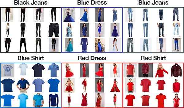
Our dataset consists of 2,167 images across six categories, including:
- Black jeans (344 images)
- Blue dress (386 images)
- Blue jeans (356 images)
- Blue shirt (369 images)
- Red dress (380 images)
- Red shirt (332 images)
The goal of our Convolutional Neural network will be to predict both color and clothing type.
I created this dataset by following my previous tutorial on How to (quickly) build a deep learning image dataset.
The entire process of downloading the images and manually removing irrelevant images for each of the six classes took approximately 30 minutes.
When trying to build your own deep learning image datasets, make sure you follow the tutorial linked above — it will give you a huge jumpstart on building your own datasets.
Multi-label classification project structure
Go ahead and visit the “Downloads” section of this blog post to grab the code + files. Once you’ve extracted the zip file, you’ll be presented with the following directory structure:
In the root of the zip, you’re presented with 6 files and 3 directories.
The important files we’re working with (in approximate order of appearance in this article) include:
- search_bing_api.py: This script enables us to quickly build our deep learning image dataset. You do not need to run this script as the dataset of images has been included in the zip archive. I’m simply including this script as a matter of completeness.
- train.py: Once we’ve acquired the data, we’ll use thetrain.pyscript to train our classifier.
- fashion.model: Ourtrain.pyscript will serialize our Keras model to disk. We will use this model later in theclassify.pyscript.
- mlb.pickle: A scikit-learnMultiLabelBinarizerpickle file created bytrain.py— this file holds our class names in a convenient serialized data structure.
- plot.png: The training script will generate aplot.pngimage file. If you’re training on your own dataset, you’ll want to check this file for accuracy/loss and overfitting.
- classify.py: In order to test our classifier, I’ve writtenclassify.py. You should always test your classifier locally before deploying the model elsewhere (such as to an iPhone deep learning app or to a Raspberry Pi deep learning project).
The three directories in today’s project are:
- dataset: This directory holds our dataset of images. Each class class has its own respective subdirectory. We do this to (1) keep our dataset organized and (2) make it easy to extract the class label name from a given image path.
- pyimagesearch: This is our module containing our Keras neural network. Because this is a module, it contains a properly formatted__init__.py. The other file,smallervggnet.pycontains the code to assemble the neural network itself.
- examples: Seven example images are present in this directory. We’ll useclassify.pyto perform multi-label classification with Keras on each of the example images.
If this seems a lot, don’t worry! We’ll be reviewing the files in the approximate order in which I’ve presented them.
Our Keras network architecture for multi-label classification
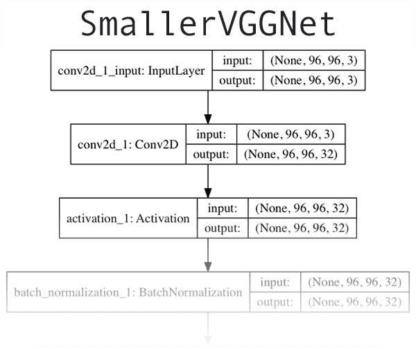
The CNN architecture we are using for this tutorial is
As a matter of completeness we are going to implement
Ensure you’ve used the “Downloads” section at the bottom of this blog post to grab the source code + example images. From there, open up the
On Lines 2-10, we import the relevant Keras modules and from there, we create our
Our class is defined on Line 12. We then define the
The
The optional argument,
Keep in mind that this behavior is different than our original implementation of
From there, we enter the body of
Let’s build the first
Our
Dropout is the process of randomly disconnecting nodes from the current layer to the next layer. This process of random disconnects naturally helps the network to reduce overfitting as no one single node in the layer will be responsible for predicting a certain class, object, edge, or corner.
From there we have two sets of
Notice the numbers of filters, kernels, and pool sizes in this code block which work together to progressively reduce the spatial size but increase depth.
These blocks are followed by our only set of
Fully connected layers are placed at the end of the network (specified by
Line 65 is important for our multi-label classification —
Implementing our Keras model for multi-label classification
Now that we have implemented
I urge you to review the previous post upon which today’s
Open up
On Lines 2-19 we import the packages and modules required for this script. Line 3 specifies a matplotlib backend so that we can save our plot figure in the background.
I’ll be making the assumption that you have Keras, scikit-learn, matpolotlib, imutils and OpenCV installed at this point.
If this is your first deep learning rodeo, you have two options to ensure you have the proper libraries and packages ready to go:
- Pre-configured environment (you’ll be up and running in less than 5 minutes and you can train today’s network for less money than a cup of Starbucks coffee)
- Build your own environment (requires time, patience, and persistence)
I’m a fan of pre-configured environments in the cloud that you can spin up, upload files, train + grab your data, and then terminate in a matter of minutes. The two pre-configured environments I recommend are:
- Pre-configured Amazon AWS deep learning AMI with Python
- Microsoft’s data science virtual machine (DSVM) for deep learning
If you insist on setting up your own environment (and you have time to debug and troubleshoot), I suggest that you follow any of the following blog posts:
- Configuring Ubuntu for deep learning with Python (CPU only)
- Setting up Ubuntu 16.04 + CUDA + GPU for deep learning with Python (GPU and CPU)
- macOS for deep learning with Python, TensorFlow, and Keras
Now that (a) your environment is ready, and (b) you’ve imported packages, let’s parse command line arguments:
Command line arguments to a script are like parameters to a function — if you don’t understand this analogy then you need to read up on command line arguments.
We’re working with four command line arguments (Lines 23-30) today:
- --dataset: The path to our dataset.
- --model: The path to our output serialized Keras model.
- --labelbin: The path to our output multi-label binarizer object.
- --plot: The path to our output plot of training loss and accuracy.
Be sure to refer to the previous post as needed for explanations of these arguments.
Let’s move on to initializing some important variables that play critical roles in our training process:
These variables on Lines 35-38 define that:
- Our network will train for 75 EPOCHSin order to learn patterns by incremental improvements via backpropagation.
- We’re establishing an initial learning rate of 1e-3(the default value for the Adam optimizer).
- The batch size is 32. You should adjust this value depending on your GPU capability if you’re using a GPU but I found a batch size of32works well for this project.
- As stated above, our images are 96 x 96and contain3channels.
Additional detail is provided in the previous post.
From there, the next two code blocks handle loading and preprocessing our training data:
Here we are grabbing the
Next, we’re going to loop over the
First, we load each image into memory (Line 53). Then, we perform preprocessing (an important step of the deep learning pipeline) on Lines 54 and 55. We append the
Lines 60 and 61 handle splitting the image path into multiple labels for our multi-label classification task. After Line 60 is executed, a 2-element list is created and is then appended to the labels list on Line 61. Here’s an example broken down in the terminal so you can see what’s going on during the multi-label parsing:
As you can see, the
We’re not quite done with preprocessing:
Our
We also convert labels to a NumPy array as well.
From there, let’s binarize the labels — the below block is critical for this week’s multi-class classification concept:
In order to binarize our labels for multi-class classification, we need to utilize the scikit-learn library’s MultiLabelBinarizer class. You cannot use the standard
Here’s an example showing how
One-hot encoding transforms categorical labels from a single integer to a vector. The same concept applies to Lines 16 and 17 except this is a case of two-hot encoding.
Notice how on Line 17 of the Python shell (not to be confused with the code blocks for
Let’s construct the training and testing splits as well as initialize the data augmenter:
Splitting the data for training and testing is common in machine learning practice — I’ve allocated 80% of the images for training data and 20% for testing data. This is handled by scikit-learn on Lines 81 and 82.
Our data augmenter object is initialized on Lines 85-87. Data augmentation is a best practice and a most-likely a “must” if you are working with less than 1,000 images per class.
Next, let’s build the model and initialize the Adam optimizer:
On Lines 92-95 we build our
From there, we’ll compile the model and kick off training (this could take a while depending on your hardware):
On Lines 105 and 106 we compile the model using binary cross-entropy rather than categorical cross-entropy.
This may seem counterintuitive for multi-label classification; however, the goal is to treat each output label as an independent Bernoulli distribution and we want to penalize each output node independently.
From there we launch the training process with our data augmentation generator (Lines 110-114).
After training is complete we can save our model and label binarizer to disk:
From there, we plot accuracy and loss:
Accuracy + loss for training and validation is plotted on Lines 127-137. The plot is saved as an image file on Line 138.
In my opinion, the training plot is just as important as the model itself. I typically go through a few iterations of training and viewing the plot before I’m satisfied to share with you on the blog.
I like to save plots to disk during this iterative process for a couple reasons: (1) I’m on a headless server and don’t want to rely on X-forwarding, and (2) I don’t want to forget to save the plot (even if I am using X-forwarding or if I’m on a machine with a graphical desktop).
Recall that we changed the matplotlib backend on Line 3 of the script up above to facilitate saving to disk.
Training a Keras network for multi-label classification
Don’t forget to use the “Downloads” section of this post to download the code, dataset, and pre-trained model (just in case you don’t want to train the model yourself).
If you want to train the model yourself, open a terminal. From there, navigate to the project directory, and execute the following command:
As you can see, we trained the network for 75 epochs, achieving:
- 98.57% multi-label classification accuracy on the training set
- 98.42% multi-label classification accuracy on the testing set
The training plot is shown in Figure 3:

Applying Keras multi-label classification to new images
Now that our multi-label classification Keras model is trained, let’s apply it to images outside of our testing set.
This script is quite similar to the
When you’re ready, open create a new file in the project directory named
On Lines 2-9 we
Then we proceed to parse our three required command line arguments on Lines 12-19.
From there, we load and preprocess the input image:
We take care to preprocess the image in the same manner as we preprocessed our training data.
Next, let’s load the model + multi-label binarizer and classify the image:
We load the
From there we classify the (preprocessed) input
- Sorting the array indexes by their associated probability in descending order
- Grabbing the first two class label indices which are thus the top-2 predictions from our network
You can modify this code to return more class labels if you wish. I would also suggest thresholding the probabilities and only returning labels with > N% confidence.
From there, we’ll prepare the class labels + associated confidence values for overlay on the output image:
The loop on Lines 44-48 draws the top two multi-label predictions and corresponding confidence values on the
Similarly, the loop on Lines 51 and 52 prints the all the predictions in the terminal. This is useful for debugging purposes.
Finally, we show the
Keras multi-label classification results
Let’s put
Let’s try an image of a red dress — notice the three command line arguments that are processed at runtime:

Success! Notice how the two classes (“red” and “dress”) are marked with high confidence.
Now let’s try a blue dress:

A blue dress was no contest for our classifier. We’re off to a good start, so let’s try an image of a red shirt:
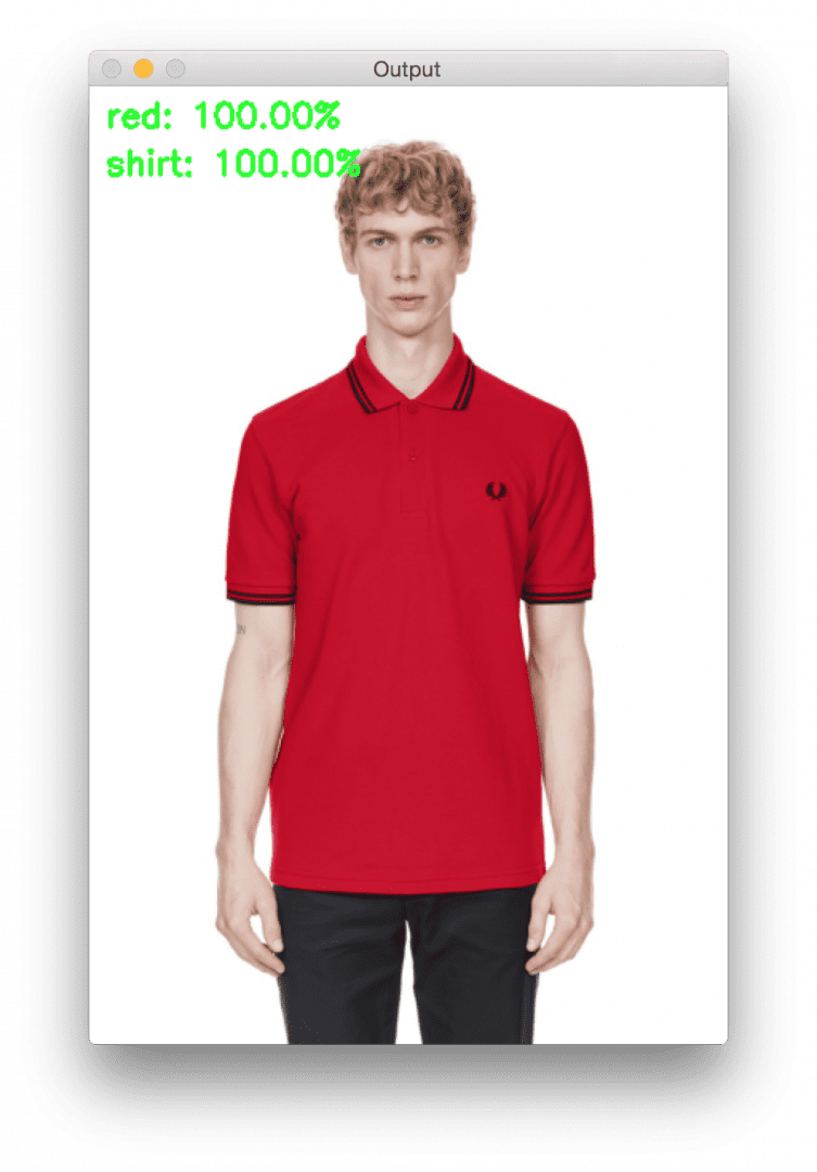
The red shirt result is promising.
How about a blue shirt?
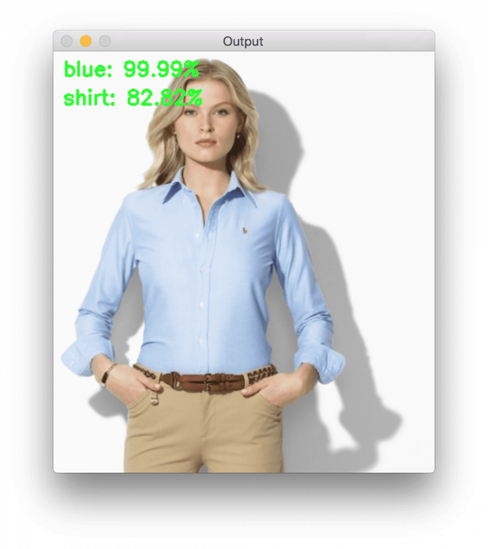
Our model is very confident that it sees blue, but slightly less confident that it has encountered a shirt. That being said, this is still a correct multi-label classification!
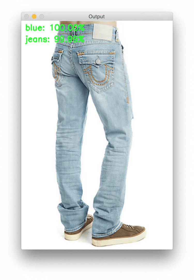
Let’s see if we can fool our multi-label classifier with blue jeans:
Let’s try black jeans:
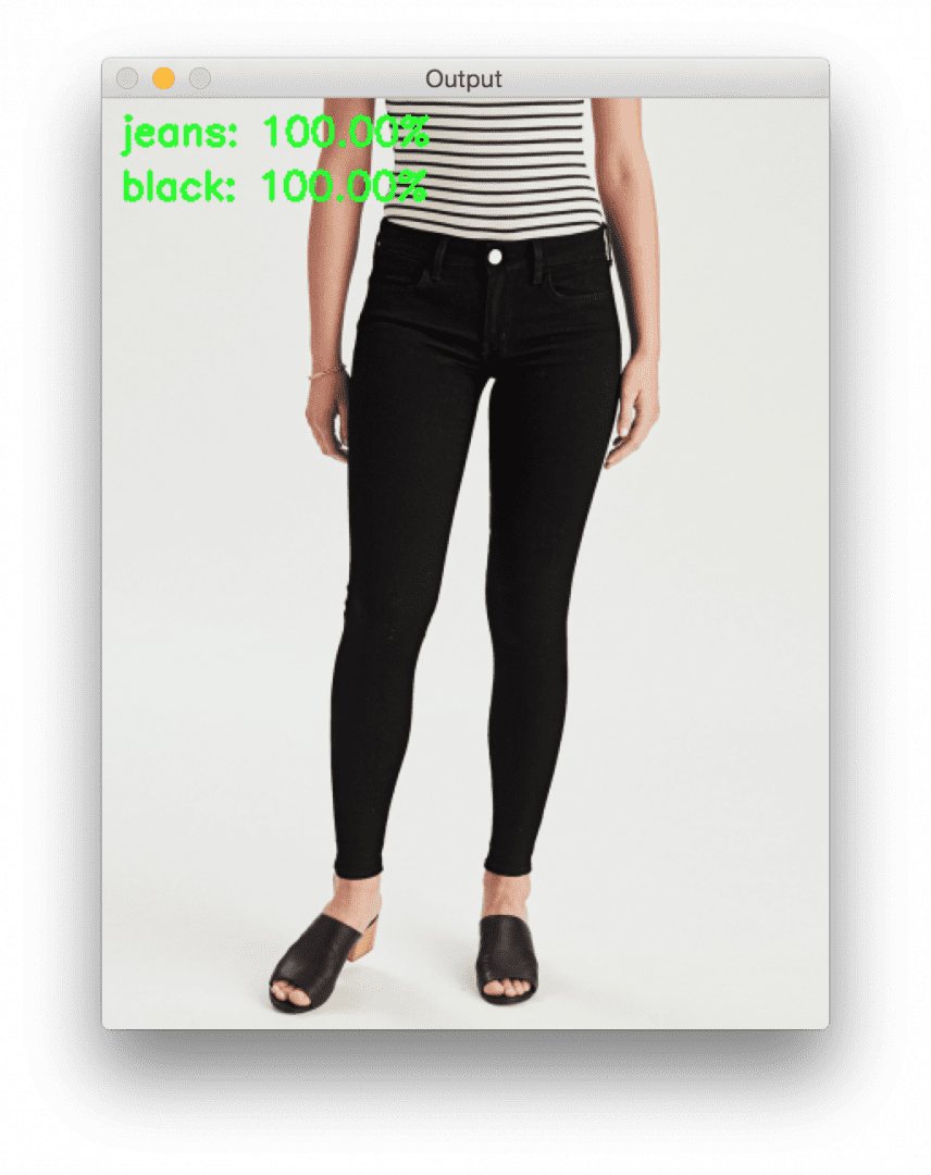
I can’t be 100% sure that these are denim jeans (they look more like leggings/jeggings to me), but our multi-label classifier is!
Let’s try a final example of a black dress (
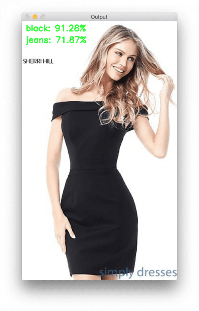
Oh no — a blunder! Our classifier is reporting that the model is wearing black jeans when she is actually wearing a black dress.
What happened here?
Why are our multi-class predictions incorrect? To find out why, review the summary below.
Summary
In today’s blog post you learned how to perform multi-label classification with Keras.
Performing multi-label classification with Keras is straightforward and includes two primary steps:
- Replace the softmax activation at the end of your network with a sigmoid activation
- Swap out categorical cross-entropy for binary cross-entropy for your loss function
From there you can train your network as you normally would.
The end result of applying the process above is a multi-class classifier.
You can use your Keras multi-class classifier to predict multiple labels with just a single forward pass.
However, there is a difficulty you need to consider:
You need training data for each combination of categories you would like to predict.
Just like a neural network cannot predict classes it was never trained on, your neural network cannot predict multiple class labels for combinations it has never seen. The reason for this behavior is due to activations of neurons inside the network.
If your network is trained on examples of both (1) black pants and (2) red shirts and now you want to predict “red pants” (where there are no “red pants” images in your dataset), the neurons responsible for detecting “red” and “pants” will fire, but since the network has never seen this combination of data/activations before once they reach the fully-connected layers, your output predictions will very likely be incorrect (i.e., you may encounter “red” or “pants” but very unlikely both).
Again, your network cannot correctly make predictions on data it was never trained on (and you shouldn’t expect it to either). Keep this caveat in mind when training your own Keras networks for multi-label classification.
Comments
Post a Comment