MSE Vs Entropy

A loss function is a parameter estimation function which represents the error (loss) of a machine learning (ML) model. The main goal of every ML model is to minimize this error. Loss basically represents some numerical value that tells us how poor the prediction is, considering only one example. In case the prediction is ideal, the loss is going to be 0. In other cases, the prediction is not that good, so the model's loss/error is (much) higher. A loss function is also called "cost function", "objective function", "optimization score function" or just "error function". So don't get confused! 😀

A loss function is a useful tool with the means of which we can estimate weights and biases that suit the model in the best way. By finding the most appropriate parameters for a ML model, the model will then have a low error in respect to all data samples in the dataset.

The function is called "loss" because it penalizes the model if it produces a false or not optimal prediction. A loss function "punishes" the model according to its predictions in a way that the model receives a "feedback" to some extent from the loss function and can improve on it further.

In short, the major task of a loss function is to determine the most optimal gradients (vectors with partial derivatives) in a ML model, so it can help to minimize the error. This is our "goal", our "ideal outcome" we actually want to have for our model and we try to make what we have as an output as close to that "ideal outcome" as possible with the help of a loss function. We can achieve this optimal, desired outcome for our model by adjusting weights and biases: our model's parameters. Therefore, we call loss fucntions "parameter estimation functions".

There are many loss functions out there. You can look at some of them, already implemented in Tensorflow: tf.losses .

Homer Simpson Math 😃

And now we will go through some frequently used loss functions.

Squared Error

As an example of loss functions, we will look at the squared error function, which is widely used in linear regression. The error will be larger in case, when the prediction is far away from the desired goal.

Likelihood (L) = Σ Ni=1 (desired_outputi - predicted_outputi)2

or to make it shorter:

= Σ Ni=1 (di - pi)2

Mean Squared Error (MSE)

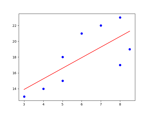
MSE determines how close some line (e.g. a regression line) is to some data sample set. MSE measures the distances from those data samples up to the line. These distances are called the errors, which MSE squares in the end. We have to square the errors (distances) because we might encounter negative values otherwise. The larger the differences between a data point and its projection on the line, the more importance it gains.

Mean Squared Error has the "mean" part in its name because we find the average of some error set (the distances) in the end of the computation. MSE again operates as estimator for model's performance. Look again at the Squared Error formula above and proceed with this one:

Notice that this function is a quadratic one. That means this function is a convex function. A convex function has one global minimum. Such quality is rather helpful because our computation won't get stuck in a local minimum.

If the value of MSE is small, it denotes that we are close to find the best fit for the line. So, the smaller the value, the better fit it means. Because of the quadratic element in the formula, one should always remember that MSE highlights the extremes in its calculations.

The algorithm of the MSE:

1. find the regression line for the data set

2. use the formula of MSE: find the error (the distances), square the errors, sum the errors up, find the mean.

Maximum Likelihood Estimation

or MLE for short, is a function applied for parameter estimation. In MLE the loss function is represented as the log-likelihood function. Log-likelihood is used to derive the maximum likelihood of some parameter Θ (theta). We use log here because the asymptotic curve of the logarithm prevents from exploding or shirking values. Thus the sums of the values are easier to analyze.

In models, based on probability, MLE has a nice application in relation to loss functions as MLE can be used to figure out the loss function for such models. Thus, maximum likelihood estimation can be applied to select a loss function for a ML model.

You can read more about Maximum Likelihood Estimation in the end of this article .

Cross Entropy

Cross Entropy Loss (sometimes named "Log Loss" or "Negative Log Likelihood") is one of the loss functions in ML. It judges a probability output of a ML classification model, that lies between [0;1]. We normally use cross entropy as a loss function when we have the softmax activation function in the last output layer in a multi layered neural network. In case that the predicted probability continuously varies from the actual label, the cross entropy will increase. In the ideal situation the cross entropy (or log loss) is equal to zero, so the difference from the actual (ideal) label is zero (or very small).

As a rule of thumb, use the cross entropy loss with softmax.

The idea of cross entropy and entropy itself roots in the information theory which deals with the problem of reliable message transmission with zero or minimum amount of information loss. We also want only useful information, with which we can make further predictions.

In other words, entropy is a measure of practical information we receive from one data point. The entropy becomes large if the variation in the data becomes large.

Binary Cross Entropy vs Categorical Cross Entropy

Binary Cross Entropy Function :

If we have to classify only two classes, we chose binary cross entropy.

L = - Σ Nn=1 {dn log pn + (1 - dn) log(1 - pn)}

We said before that we use softmax as an activation function in the last layer. With binary cross entropy, it is advisable to use the sigmoid activation function. Feel free to read more about activation functions.

The code demonstration will be done with the help of the Keras ML library.

from keras.preprocessing import sequence
from keras.models import Sequential
from keras.layers import Dense, Embedding, LSTM, Bidirectional


#  this function builds, trains and evaluates a keras LSTM model 

def build_and_evaluate_model(x_train, y_train, x_develop, y_develop):

    x_train = sequence.pad_sequences(x_train, maxlen = 100)
    x_dev = sequence.pad_sequences(x_develop, maxlen = 100)
    
    model = Sequential()
    model.add(Embedding(input_dim = 10000, output_dim = 50))  #input_dim or the size of the data set, e.g vocabulary 
    model.add(Bidirectional(LSTM(units = 25)))
    model.add(Dense(1,activation='sigmoid'))
    model.predict(x_develop)
    model.compile(loss = 'binary_crossentropy', optimizer = 'adam', metrics=['accuracy'])
    model.fit(x = x_train, y = y_train, batch_size = 32, epochs = 10, validation_data = (x_develop, y_develop))
    
    score, acc = model.evaluate(x_develop, y_develop)
 
    return score, acc, model 

Consider the whole code following this link to: Train a recurrent convolutional network on the IMDB sentiment classification task.

To find out more about the LSTM model used in the code above, read this article.

Categorical Cross Entropy Function :

If we have to classify multiple classes, we chose categorical cross entropy.

Categorical Cross Entropy is sometimes referred to as the softmax loss. The softmax loss is basically the softmax activation function combined with the cross entropy loss function. Essentially, it will output some probability over some N classes for each data sample.

Categorical Cross Entropy is already implemented in the Keras ML library:

keras.losses.categorical_crossentropy(y_true, y_pred, from_logits=False, label_smoothing=0) 

We can also use already implemented in Keras mean squared error (MSE) as our loss function. As a general rule, use a linear activation function and only one node in the output layer if MSE is used :

model.compile(loss="mse")  #instead of writing "mse", "mean_squared_error" is also acceptable and less cryptic 

model.add(Dense(1, activation="linear"))

Feel free to consult the Keras official documentation .

Conclusion

To sum up, loss functions are not always easy to comprehend. In some ML cases, it is more relevant to measure and present the accuracy of classification Ml models.

Sometimes we should select other metrics than the loss functions. An important thought: one may assume that the ML model which has the minimum loss, would be the best pick, but it doesn't have to be like this. The model with the lowest loss still can be the model with the worst metric after all.

A sufficient practice would be to apply a loss function for evaluation of the model's learning progress. Shortly, use loss functions for optimization: analyze whether there are typical problems such as: slow convergence or over/underfitting in the model. Chose the proper metric according to the task the ML model have to accomplish and use a loss function as an optimizer for model's performance.